Santa Fe DataBase Solutions

• FastTrack |
• Technology |
• Licensing |
• Contact |
• Site Map

PATH // www.sfdbs.com > FastTrack

FastTrack

For the database professional -- what this website is all about.

This section is intended for database experts with in depth knowledge of relational database technology and ongoing, hands-on experience designing and deploying databases. It would also be advantageous if you are familiar with a scripting language (like Tcl or Perl) with ODBC extension.

Background: Conventional Relationship Representations

We assume every database designer who ever translated an E-R, UML or other database design into SQL is already familiar with the following two ways to represent relationships in relational databases:

Figure 1. The PKFK (Primary Key / Foreign Key) Representation

Figure 2. The JT (Junction Table) Representation

The diagrams to the left show relations in the ER (Entity-Relationship) style with arrows indicating relationships. The diagrams to the right show key and non-key schema attributes with arrows indicating foreign key to primary key references.

There doesn't seem to be any commonly accepted name for the Figure 1 representation. We call it the PKFK (for Primary Key / Foreign Key) representation or just PKFK. PKFK demonstrates the fundamental construction for tuple-tuple relationships: A relationship instance between parent tuple and child tuples is represented by storing the value of the primary key attribute (Parent_pk) of the Parent relation tuple as the value of a foreign key attribute (Child_Parent_fk) in the Child relation tuple. (Parent and Child relations may be the same.) Using this representation, application of the relational equijoin operator to the Parent- and Child relations on attributes Parent_pk and Child_Parent_fk retrieves all related parent-child tuple pairs. PKFK is the most primitive form of this fundamental relationship construction.

With a single foreign key, a Child tuple in PKFK can be related to at most one (or if NULL values are prohibited, exactly one) Parent tuple. But unless prohibited (by a UNIQUE integrity constraint on Child_Parent_fk), more than one Child tuple can be related to ("share") the same Parent tuple. Relationships represented using PKFK are called "one-to-many" -- one parent, many childs (children!). PKFK possesses a kind of representational elegance and is very space efficient.

Sometimes a database design calls for a Parent-Child relationship in which many Parent tuples can be related to one Child tuple and many Child tuples can be related to the same Parent tuple. Common practice for representing such "many-to-many" relationships is to define a specialized relation that combines two PKFK representations, one for relating a tuple in this relation to one tuple in the Parent relation, and a second to relate it to one tuple in the Child relation. The combination is interpreted as a bipartite relation between tuples of Parent and tuples of Child. This representation is depicted in Figure 2. The specialized relation is variously referred to as a "junction table" or "association table." We'll refer to this as the JT (for Junction Table) representation.

In our formulation, the junction relation schema consists of only a primary key and two foreign keys, no attribute data. The primary key (Jnct_pk) can be omitted if the composite key (Jnct_Parent_fk,Jnct_Child_fk) is declared as the primary key. A relation whose schema consists exclusively of primary- and foreign key attributes is called a structure relation.

CONVENTION: For ease of exposition, we use the following notational conventions: Attribute names with suffixes "_pk" and "_fk" designate primary key and foreign key attributes respectively. If XXX is a relation, XXX_pk is its primary key. If XXX is the Parent relation in a PKFK representation and YYY the Child relation, the child relation foreign key is YYY_XXX_fk.

What are PKFK and JT?

PKFK and JT are relational database data structures -- that is, data structures used to organize data within relational databases. Relational database data structures should not be confused with file data structures (like B-trees, etc.) used to implement relations, indexes, etc. in relational database management systems (RDBMS).

We refer to PKFK and JT as foreign key database data structures to differentiate them from database data structures like nested sets and nested intervals that don't rely on foreign keys. (Nested set and nested interval representations are intra-relational, not inter-relational. These representations rely on interval arithmetic instead of the equijoin mechanism to logically resolve parent-child relationships.) Non-foreign key data structures are are not discussed further in these pages.

PKFK and JT are ubiquitous. Together they probably account for 99% of all relationship representations in all databases in a ratio of about 80/20, PKFK to JT. Every non-trivial database employs one or the other or both. There are other foreign key database data structures besides PKFK and JT. They can be characterized by relation schemas that combine two or more foreign key attributes with at least one non-key attribute. For now, we will ignore all these "other" representations.

The Aggregate-Link Database Data Structure

Figure 3 depicts something new -- the Aggregate-Link database data structure for representing relationships.

Figure 3. The A-L (Aggregate-Link) Representation

Inspection of Figure 3 shows how a relationship between tuples in a Parent relation and tuples in a Child relation is represented by the Aggregate-Link (A-L) schema. The representation requires two structure relations, Aggregate and Link. One Aggregate tuple represents ("reifies") an aggregation and identifies the Parent tuple by its primary key value Parent_pk stored in foreign key attribute Aggregate_Parent_fk. Each Link tuple identifies one Child tuple by the Child tuple's primary key value Child_pk stored in foreign key attribute Link_Child_fk, and associates it (via Link_Aggregate_fk) with one aggregation -- i.e., one Aggregate tuple. (Yes, PKFK is used to relate the Aggregate- and Link relations and yes, referential integrity from Link_Aggreggate_fk to Aggregate_pk should be specified to prevent unassociated Link tuples. One way to regard the construction is as a PKFK relationship in which the Parent and Child tuples are replaced by their primary keys acting as indirect references.) The Aggregate and Link structure relations are a unit: They are created, used and destroyed together as a matching pair. Individually they have no intended meaning or purpose.

Like PKFK and JT, the Aggregate-Link (A-L) representation is a foreign key database data structure. And like PKFK and JT, the A-L can be used to represent relationships between tuples in a Parent relation and tuples in a Child relation. We'll compare A-L to PKFK and JT below. First, a simple example to show the A-L represention for a many-to-many Department-Employee relationship between Departments and Employees.

An Aggregate-Link Example

Here is the schema for the Department-Employee example:

Figure 4. A-L Schema for the Department-Employee example.

Here are the relations (2 entity, 2 structure) with sample data:

Here is a graphic depiction of the Department-Employee example (Figure 5).

Figure 5. Graphic Depiction for The Department-Employee Example.

See Aggregate-Link Department-Employee Example for greater detail including SQL statements to replicate the example.

Aggregate-Link Compared to PKFK and JT

With its only foreign key in an entity relation, PKFK requires no structure relation. JT requires one structure relation with two foreign keys, A-L two structure relations with three foreign keys. Most people who see A-L for the first time ask Why the Aggregate structure relation is needed at all? -- it seems to serve no purpose. But what is not obvious is how reification of the aggregation as an Aggregate tuple plus that third foreign key result in more relationship types and more precise relationship representation than PKFK and JT.

Precision

Consider the Department-Employee Example (above). Notice that Department "Personnel" (DEPT4) is referenced by AGG tuple 103, but that no aggregate tuple references Department "Projects". Similarly, LNK tuple 1007 references Employee "Jim White" (EMP16), but that no LNK tuple references "Jack Mills" (EMP17). In that sense, Department "Personnel" and Employee "Jim White" are in the relationship while Department "Projects" and Employee "Jack Mills" are not in the relationship. Further, AGG tuple 103 (for Department "Personnel") is not referenced by any LNK tuple so "Personnel" is a childless parent. And for AGG tuple 104 (referenced by the LNK tuple 1007 for "Jim White"), AGG_DEPT_fk is NULL so that "Jim White" is an orphan. In other words, "orphans" (childs with no parent) and childless parents are explicitly represented in A-L. (By this reasoning, "Projects" and "Jack Mills" should not appear in Figure 5.)

Compare this to PKFK: Where allowed, an orphan is represented by a NULL Child_Parent_fk foreign key value. Childless parents are always allowed and are represented implicitly by the absence of reference in Child_Parent_fk among all Child tuples.

Consider JT: An orphan is represented by the absence of reference in foreign key Jnct_Child_fk among all JT tuples, a childless parent by the absence of reference in the other foreign key, Jnct_Parent_fk. Both representations are implicit.

In both PKFK and JT, the representation of orphans and childless parent allows for interpretation as as either in the relationship (think: outer join) or not in the relationship (think: inner join). But it is not possible to have some orphan child tuples in the relationship and some child tuples not in the relationship. Nor do PKFK or JT allow some childless parents in the relationship and some parent tuples not in the relationship at all. The explicit representation in A-L makes it possible to have both "in" and "not in" for both parent- and child tuples.

Richness

Relationships are classified by cardinality, an imprecise and inconsistently used term for the minimum and maximum number of child tuples related to any one parent tuple and the minimum and maximum number of parent tuples related to any one child tuple. (There is no agreed upon naming convention for cardinalities. The Object Management Group's Unified Modelling Language (UML) is an important step towards standardization for naming and graphically depicting relationship cardinalities.)

The cardinality of a relationship is specified by combinations of UNIQUE and NOT NULL integrity constraints on the foreign keys of the relationship representation. The intended cardinality is effectively achieved by RDBMS enforcement of these integrity constraints. A detailed comparison of relationship cardinalities for the three representations can be found in Relational Cardinality Types. Summarizing the main points:

• PKFK
• PKFK can represent relationships of 4 cardinalities:
  • 1-to-(0,1), 1-to-(0,M), (0,1)-to-(0,1) and (0,1)-to-(0,M).
• JT
• JT can represent relationships of 4 cardinalities:
  • (0,1)-to-(0,1), (0,1)-to-(0,M), (0,M)-to-(0,1), and (0,M)-to-(0,M).
• A-L
• A-L can represent relationships of 20 cardinalities:
  • the 6 distinct cardinalities provided by PKFK & JT
  • (1,M)-to-(0,1) and (1,M)-to-(0,M)
  • plus 12 lattice cardinalities that admit multiple aggregate tuples with the same parent and/or multiple links to the same child occurrences for one aggregation. (Lattice cardinality types cannot be expressed in our notation or UML.)

Lattice Relationships

In A-L, Child tuples are not directly linked to a Parent tuple, but to an Aggregate tuple that is linked to a Parent tuple. If Aggregate_Parent_fk is NOT UNIQUE, more than one aggregation instance can have the same Parent tuple. Similarly, if the composite key (Link_Aggregate_fk,Link_Child_fk) is NOT UNIQUE, an aggregation instance can contain multiple instances of the same Child tuple. All lattice relationships allow more than one aggregation with the same Parent tuple, or more than one Child tuple per aggregation, or both.

Figure 6 depicts a simple example of a lattice relationship. Suppose person A is parent to 5 children, {B,C,D,E,F}, two {B,C} with one partner and three {D,E,F} with a second partner. This is represented in A-L with A as parent in two aggregations. Note how the "half-sibling" relationship is preserved.

Figure 6. An Example of a Lattice Relationship.

If we attempt to represent Figure 6 using PKFK or JT, the result is the following (incorrect) interpretation (Figure 7) in which the half-sibling relationship has been lost:

Figure 7. Incorrect PKFK or JT Representation of a Lattice.

The Aggregate-Link schema supports 12 different lattice relationships. The value of these A-L lattice relationships for modeling has not been explored. They seem to suggest decision support.

Performance

Figure 8 shows the relations and relationships of PKFK, JT and A-L:

Figure 8. PKFK, JT and A-L.

Your intuition is correct if it tells you the following about the relative performance of these 3 representations in SQL Select queries:

• PKFK representation (with one join) is fastest
• A-L (with three joins) the slowest
• JT (with two joins) is somewhere in between

Historically, performance optimization has been an important area of database research that has led to improved representations and faster query processing. Performance optimization for the A-L representation has not been explored.

Structure Independence

In PKFK, the lone foreign key attribute is part of the Child relation schema so that a Child tuple represents both a child entity and the relationship to a parent entity. In JT, the two foreign keys are in a separate structure relation, not the entity relations. In other words, the JT represention models the structure of the relationship independent of either entity relation. We refer to this property as Structure Independence. A-L is also structure independent.

Structure independence has a subtle, temporal quality: A relationship implemented using a structure independent representation can be superimposed over entity relations after they have been populated without schema modification to entity relations. PKFK is not structure independent. In current usage, structure independence is probably unimportant because OLTP database schemas evolve slowly (if at all). And the choice of JT over PKFK is dictated only by the need for a many-to-many relationship, not to position foreign keys in structure relations instead of entity relations. Nevertheless, modifying the schema of a populated database by adding structure dependent PKFK relationship representations almost always requires database restructuring. Adding a relationship using a structure independent representation does not.

If creation and destruction of relationships are common occurrences, they must be lightweight processes. Under these circumstances, structure dependent PKFK would be the worst representational choice for new relationships. JT is structure independent, but then so is A-L. With more relationship cardinality types and greater precision, A-L is far better suited to relationship representation in this environment (i.e., frequent relationship creation/destruction) than JT. Even where relationship creation/destruction are uncommon, a structure independent representation implies that entity update transactions and relationship update transactions cannot block one another.

The Use of Aggregate-Link in Conventional OLTP Databases

The Aggregate-Link representation of relationship is a foreign key database data structure that compares favorably to conventional representations with respect to precision and richness, but not performance:

• Explicit relationship representation in A-L provides greater precision than conventional representations (PKFK&JT).
• A-L provides a richer collection of relationship types ("cardinalities") than conventional representations (PKFK&JT) including new, lattice relationships.
• A-L is NOT more performant than conventional representations (PKFK&JT).
• Structure Independence in A-L isolates structure representation from entity representation (PKFK).

Combining Aggregate-Link with PKFK and JT in OLTP databases.

The potential for using A-L together with PKFK and JT is limited:

• Although A-L provides every relationship cardinality type available with PKFK and JT, adding it to the database designer's toolkit adds complexity and may degrade performance.
• Structure independent A-L allows for creating, populating, analyzing and destroying relationships without impact on existing relations and relationship structures. This may prove useful for analyzing entity attribute values and existing relationships. (For example: Is a given attribute a candidate key? Does a junction table in fact represent a 1-to-M relationship?)
• The lattice relationship types provided by A-L may enable new decision support applications within existing databases. Practical uses for lattice relationships have not been explored.

Using Aggregate-Link exclusively in OLTP databases.

A-L can precisely replace both PKFK and JT and can be defined with referential integrity. Conventional OLTP databases could therefore be constructed using only A-L, no PKFK or JT. The resulting database has several interesting properties, not the least of which is a logical partitioning of database relations into entity relations and structure relations. The following are advantages A-L offers in specialized databases:

• In analytic environments where the entity relations and relationships of the database schema are continually evolving, A-L's structure independent representation allows addition or deletion of relationships without the need for database restructuring.
• When the transaction "mix" includes updates to both entities and relationships, A-L's isolation of structure from data implies that entity updates and relationship updates are independent and can proceed without blocking one another.
• From an engineering perspective, A-L's comprehensive relationship representation simplifies database schema generation and makes multirelation SQL Select queries more uniform. In turn, this makes it easier to provide higher-level end user interfaces including named relationships.

In this FastTrack thread, we are more concerned with exploiting the Aggregate-Link representation to provide new data management capabilities than using it within conventional OLTP databases.

Aggregate-Link Structure Isolation

Beginning with the introduction of the Relational Model in 1970 [Codd 1970], all approaches to relational system design have been entity oriented -- that is, oriented to the representation of entities. Relationships are unnamed and for the most part, invisible. Yet relationships provide the structure that associates tuples in one relation to tuples in another. The join operator is the principal means for retrieving related tuples and their attribute data. Relationships have never been treated as first-class components.

The Aggregate-Link representation provides a method for elevating relationships to first-class, named status. Intuitively, this would be achieved by extending SQL with DDL (Data Definition Language) syntax for creating named relationships and DML (Data Manipulation Language) syntax for update and retrieval. Unfortunately, SQL is already so complex that few SQL experts fully exploit all its features. Integrating relationship constructs and operators would therefore make the SQL language even more complex, something the ANSI SQL standardization committees would almost certainly resist.

There is however another, semi-transparent means of working the Aggregate-Link representation into SQL without change. (That is, entity oriented.) The following example illustrates how structure independence not only isolates structure representation from entity representation, it also isolates the query processing for structure from query processing for entities:

Example of Structure Isolation

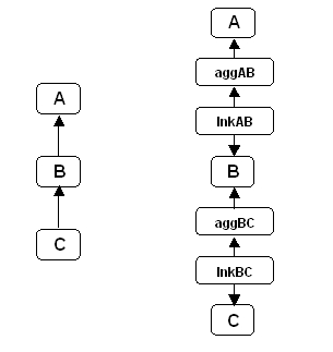
Suppose we have 3 relations, A, B and C connected by two relationships, one between A and B, the other between B and C. Figure 9 illustrates this on the left as an ER diagram and on the right as a schema diagram:

Figure 9. ER and Schema Diagrams for Relations A, B and C.

The following SQL statement retrieves attributes from A, B and C for all related triples (a,b,c) in AxBxC.

Query 1: Select A, B and C attributes for (a,b,c) in A x B x C:
select <A attributes>, <B attributes>, <C attributes>
from    A, aggAB, lnkAB, B, aggBC, lnkBC, C
where  A_pk       = aggAB_A_fk
  and  aggAB_pk   = lnkAB_aggAB_fk
  and  lnkAB_B_fk = B_pk
  and  B_pk       = aggBC_B_fk
  and  aggBC_pk   = lnkBC_aggBC_fk
  and  lnkBC_C_fk = C_pk

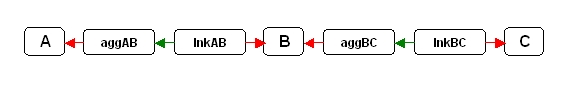
Query 1 is straightforward. In Figure 9, three entity relations (A, B, C) are related ("connected") by two pairs of Aggregate/Link structure relations (aggAB and lnkAB, aggBC and lnkBC). The intuitive way to retrieve A-, B- and C attributes is a Select query with 6 joins over the seven relations. Each predicate conjunct corresponds to an individual join. Notice that there are two distinctly different kinds of join involved: The join predicates in red are structure-to-entity relation joins, the join predicates in green are structure-to-structure relation joins. Both kinds of join predicate involve a foreign key and a primary key. Figure 10 shows this query diagrammatically with color coded arrows corresponding to the join predicates in Query 1:

Figure 10. Query 1.

Query 2 is identical to Query 1 except the terms of two structure-to-entity predicate conjuncts have been reversed and the conjuncts are grouped by the two kinds of join (red for structure-to-entity, green for structure-to-structure):

Query 2: Select A, B and C attributes for related (a,b,c) in A x B x C:
select <A attributes>, <B attributes>, <C attributes>
from   A, aggAB, lnkAB, B, aggBC, lnkBC, C
where  aggAB_pk   = lnkAB_aggAB_fk
  and  aggBC_pk   = lnkBC_aggBC_fk
  and  aggAB_A_fk = A_pk
  and  lnkAB_B_fk = B_pk
  and  aggBC_B_fk = B_pk
  and  lnkBC_C_fk = C_pk

Notice that the predicate fragment

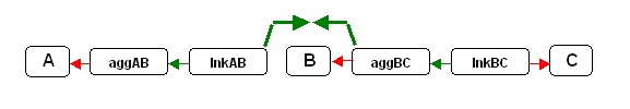
Query 3: Select A, B and C attributes for related (a,b,c) in A x B x C:
select <A attributes>, <B attributes>, <C attributes>
from   A, aggAB, lnkAB, B, aggBC, lnkBC, C
where  aggAB_pk   = lnkAB_aggAB_fk
  and  lnkAB_B_fk = aggBC_B_fk
  and  aggBC_pk   = lnkBC_aggBC_fk
  and  aggAB_A_fk = A_pk
  and  aggBC_B_fk = B_pk
  and  lnkBC_C_fk = C_pk

Figure 11. Query 3.

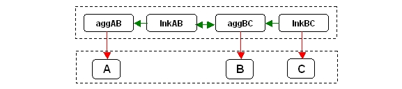
The join corresponding to the new conjunct in Query 3 is altogether different from the other kinds of join. Whereas all other joins are structure-to-structure or structure-to-entity between a foreign key and a primary key, this new join is structure-to-structure between two foreign keys, one in the Link relation of the Aggregate-Link for the A-B relationship and the other in the Aggregate relation of the Aggregate-Link for the B-C relationship. Redrawing Figure 11 with this new join represented by a green double-ended arrow, we get Figure 12.

Figure 12. Query 3.

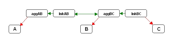
Figure 12 illustrates an important point: When using the Aggregate-Link relationship representation, a multirelation Select query can be evaluated in 2 phases, the first to resolve the structure, the second to access the attribute data. Figure 13 illustrates the evaluation strategy with all structure-to-structure relation joins in the upper dashed rectangle (first phase) and all access to entity relations in the lower dashed rectangle (second phase):

Figure 13. Isolating Structure for Relations A, B and C.

Figure 13 illustrates a pattern of structure-to-structure relation joins that generalizes for three or more entity relations related (connected) by Aggregate-Link representations.

Query 4: Select foreign keys into #temp for related (a,b,c) in A x B x C:
select aggAB_A_fk, aggBC_B_fk, lnkBC_C_fk into #temp
from   aggAB, lnkAB, aggBC, lnkBC
where  aggAB_pk   = lnkAB_aggAB_fk
  and  lnkAB_B_fk = agg_BC_B_fk
  and  aggBC_pk   = lnkBC_aggBC_fk

Query 5: Use #temp to Select A, B and C attributes:
select <A attributes>, <B attributes>, <C attributes>
from   #temp, A, B, C
where  aggAB_A_fk = A_pk
  and  aggBC_B_fk = B_pk
  and  lnkBC_C_fk = C_pk

In effect, #temp (Query 4) can be viewed as an intermediate relation consisting entirely of foreign key values organized as a tableau. Each tuple of #temp specifies one foreign key for each of A, B and C. The final result is obtained by joining #temp to A, B and C (Query 5). If there were any additional subsetting predicates over data attributes of A, B and C, these could be applied as part of the second phase.

The approach illustrated by this example generalizes to the evaluation of any multirelation Select query over n relations R₁, R₂, ..., R_n joined via n-1 relationships over (R₁, R₂), ..., (R_n-1, R_n) with foreign key to foreign key joins between the Link relation of (R_i-1, R_i) and the Aggregate relation of (R_i, R_i+1). There are of course multirelation Select queries over n relations where the relationships are "multi-legged" -- i.e., a relation may be joined to more than one Parent or more than one Child relation. (See M.M.David where multi-leg query evaluation is discussed in the context of XML.) The approach works here also, although the formalization is more complex.

Integration by Structure

Structure independence makes it possible to isolate structure and structure relation processing from entity data and entity relation processing. (Because it is structure independent, this also holds true for the JT representation, but not PKFK.) This separation of structure from data (that is, from non-key attribute data) may seem to provide nothing more than a curious way to evaluate multirelation Select queries, but it actually provides a completely new way to look at a relational database as the combination of two logically disjoint components, data plus structure. The data component consists of entity relations with no foreign key attributes, the structure component consists of structure relations with no attribute data. As the example illustrates, the structure can be resolved completely without access to any entity relation. The "structure" (in this case, #temp, the tableau of foreign keys) can then be instantiated with primary key access to the entity relations and no additional access to any structure relations. With both logical components residing in the same physical database, referential integrity can guarantee the validity of foreign key references. Without referential integrity -- i.e., between a foreign key attribute in a structure relation and the primary key of an entity relation -- structure-to-structure relation joins could include structure tuples joined via an invalid foreign key. This error would be detected during instantiation of the intermediate structure.

The scenario of both the logical data- and structure components residing in the same physical database corresponds to "Using Aggregate-Link exclusively in OLTP databases" (above). Without this co-location, referential integrity and therefore OLTP databases are not possible. However, for OLAP databases and analytic applications in general, the absence of referential integrity is not critical. Consider the following:

• Resolution of structure requires structure-to-structure relation joins. All structure relations must therefore reside in the same database and be managed as an independent, structure-only OLTP database.
• Instantiation requires no entity-to-entity relation joins. Entity relations are therefore not required to reside in the same database as one another.
• Instantiation only requires "read" access to entity relations by primary key. With a network database access protocol like ODBC, entity relations can reside in any database on any compliant network server.
• Foreign keys in entity relations in remote databases are ignored. Entity relations can therefore be part of remote OLTP databases.

We refer to this construction of a centralized structure database and decentralized entity databases as integration by structure. It does not provide true database federation because it does not support distributed transactions: Referential integrity between foreign keys in structure relations and primary keys in entity relations isn't even considered. Integration by structure is a simple view mechanism in which one centralized, OLTP relational "structure database" references relational entities in other OLTP databases. Updates to these other OLTP databases may cause foreign keys in the structure database to become stale, but this is characteristic of materialized views in general. The structure database we've described provides materialized views of structure absent any attribute data.

By using network database access and a dedicated structure database, an application can integrate part or all of one or more remote, read-only OLTP databases into a logical, local model. Only database data is included -- the report writing capabilities of an SQL RDBMS would not be available. (For example, the computation of an aggregate function like SUM would have to be computed by the application.) To obtain SQL's full report capabilities would require implementation support for integration by structure at the RDBM system level. That presents no serious challenge since the presentation layer functionality of SQL (i.e., ORDER BY, GROUP BY, aggregate functions) operates by post processing of a Select-Project-Join intermediate. (With integration by structure, an instantiated structure is essentially a Select-Project-Join.)

As formulated above, integration by structure extends RDBMS capability with a relational view mechanism over distributed databases. In keeping with the Relational Model, Aggregate-Link structure relations are sets: There is no implied order among the sets of Aggregate and/or Link relation tuples. Without an ORDER BY clause, the order of tuples returned in response to a multirelational Select query (like the Example of Structure Isolation, above) is not predictable.

What Next?

This web page has introduced Aggregate-Link (A-L), a foreign key relational database data structure based on 3 foreign keys in two physical structure relations. A-L represents the same kinds of relationships as conventional representations (PKFK&JT) except:

• In one data structure, the A-L representation generalizes all PKFK and JT relationship types ("cardinalities") and adds 12 new lattice relationships.
• A-L's explicit representation of childless parents and orphans is more precise than PKFK or JT.
• A-L is less performant than conventional representations (PKFK&JT).
• A-L's structure independent representation isolates structure representation from entity representation (relations).

• In combination with PKFK and JT in conventional OLTP databases.
• As a complete replacement for PKFK and JT in conventional OLTP databases.
• In a standalone, structure base for integrating entity relations in distributed OLTP databases into a virtual, OLAP database.

But the Aggregate-Link representation has several clear advantages over PKFK&JT. The question is, Are there better, mainstream data management uses for the Aggregate-Link representation?

The answer to this question is "what this website is all about".

Coming Attractions

In the next installment, we will explore the following:

• Rethinking the SQL paradigm:
• What makes SQL so difficult for the non-expert?
• How can the Aggregate-Link representation make relational database use easier?
• New relationship-oriented relational data models:
• A simple, relationship-oriented relational data model fully compatible with SQL.
• A new, ordered, relationship-oriented relational data model interoperable with SQL.
• New Directions:.
• Graphical database interfaces.
• The time dimension.
[ Go to top ]

Page Content first published: November 13, 2007
Page Content last updated: February 03, 2008